Automated Slope estimation using Python/ArcPy
Lakehead University Coursework 2023
Overview
This assignment presents a Python/ArcPy script designed to perform advanced geospatial analysis on slope values derived from a Digital Elevation Model (DEM) within a geodatabase. The script processes raster data to compute slope statistics and updates relevant attributes in a feature class representing Provincial Forest Types (PFTs). This analysis helps in understanding terrain characteristics across different forest types, which can be valuable for environmental management and land planning.
Objective
- Slope Calculation: Convert a DEM raster to a NumPy array, compute the slope, and save it as a new raster.
- Convert to Points: Change the slope raster into a point feature class with slope values at each point.
- Update Fields: Remove old slope fields from the fri feature class and add new fields for slope statistics.
- Analyze Statistics: Calculate and update average slope, standard deviation, and range for each PFT.
Location
The study area is located in the Provincial Forest of Ontario, approximately 40 kilometers north of Thunder Bay, at coordinates 48°38’53.2”N, 89°22’29.7”W.
Workflow
1. Input Data
I start by importing the library such as numpy for array processing, and arcpy for GIS operations, then i specify the workspace and input the DEM raster. This part Allows the user to specify Provincial Forest Type (PFT) values from the FRI feature class. 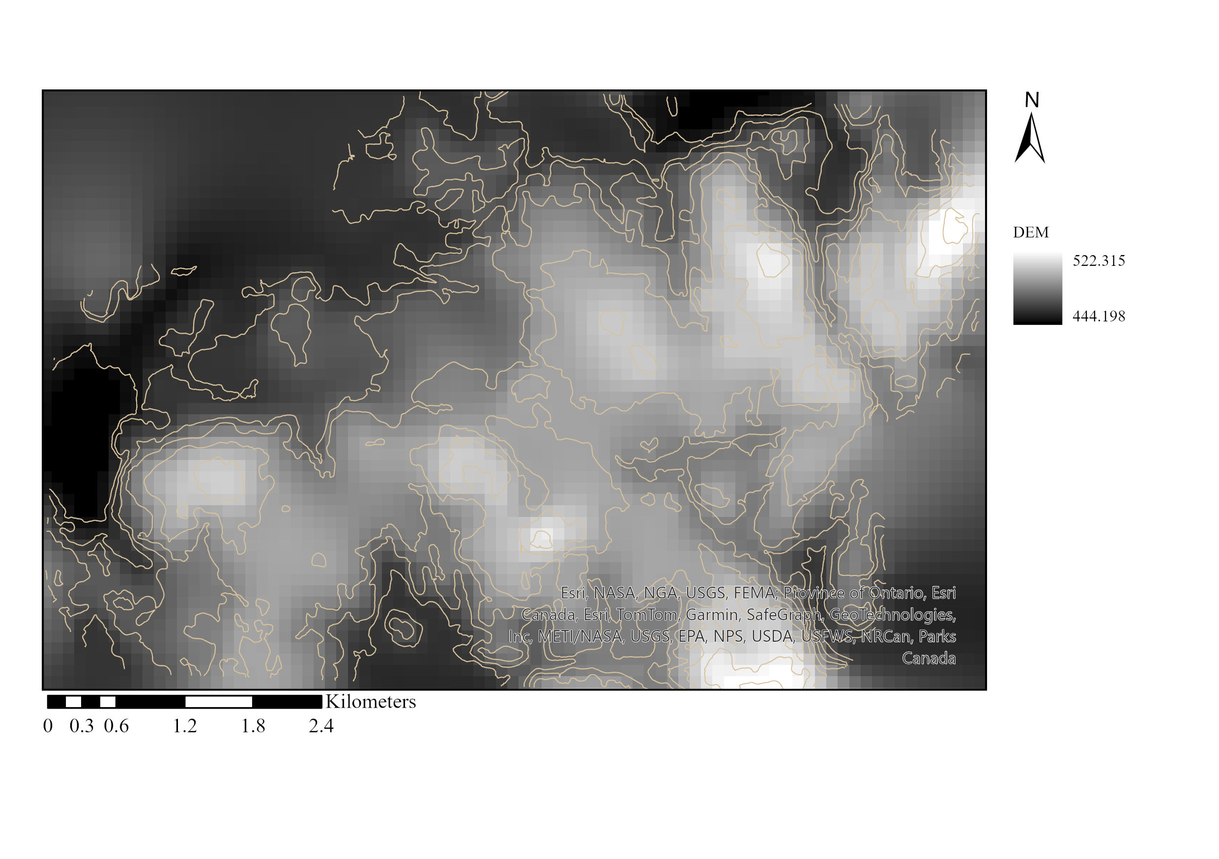 DEM data imported from jhf geodatabase
1
2
3
4
5
6
7
8
9
10
11
12
13
#~~~~~~~~~~~~~~~~~~~~~~~~~STEP 1 IMPORT LIBRARY~~~~~~~~~~~~~~~~~~~~~~~~~~~~
import numpy as np #in this case, numpy used for processing data with array
from scipy.ndimage import generic_filter # generic filter
import arcpy #arcpy used for

#~~~~~~~~~~~~~~~~~~~~~~~~~~~~STEP 2 SET PATH AND IMPORT FEATURE CLASS~~~~~~~~~~~~~~~~~~~~~
arcpy.env.workspace = r"C:\Users\Erlang\OneDrive\Documents\ArcGIS\Projects\Assignment3\data\jhf.gdb" #set the workspace path
arcpy.env.overwriteOutput = True #ensure that existing outputs are overwritten if they already exist.

input_dem = arcpy.Raster ("dem") #input dem raster feature class located inside fri geodatabase
dem = arcpy.RasterToNumPyArray (input_dem) #command used to convert a raster dataset into a NumPy array.
x_cellsize = input_dem.meanCellWidth #used to access the mean width of the cells in the raster dataset along the X-axis (columns)
y_cellsize = input_dem.meanCellHeight #used to access the mean height of the cells in the raster dataset along the Y-axis (rows
2. Slope Calculation
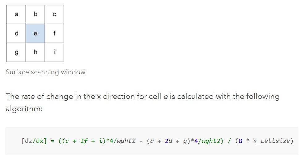 In this setup, I define a function to calculate the slope from the DEM using a 3x3 window with the planar method algorithm. The planar method in ArcPy calculates the slope by measuring the rate of elevation change over a specified horizontal distance. This approach ensures accurate slope values for each cell, which are crucial for detailed spatial analysis.
See more about slope calculation
1
2
3
4
5
6
7
8
9
10
11
12
13
14
15
16
#~~~~~~~~~~~~~~~~`STEP 3 DEFINE THE EQUATION TO CALCULATE SLOPE -(note need to reshape in array to be 3*3)~~~~~~~~~~~~~~~~~~~~
def calc_slope(input_dem, x_cellsize, y_cellsize): #the function that will be used by the generic_filter function to calculate slope values
    if -9999 in input_dem: #conditional statement This conditional statement that ensures that the calculation proceeds differently if nodata values (-9999) are present in the input array
        return -9999 # the function returns -9999 to indicate that the slope calculation couldn't be performed
    else:
        [a, b, c, d, e, f, g, h, i] = input_dem #identifiers are assigned to the positions in the used filter
        #From 3x3 box, row 1: a, b, c
        #              row 2: d, e, f
        #              row 3: g, h, i

        # Run the equation for calculating slope. See https://pro.arcgis.com/en/pro-app/tool-reference/spatial-analyst/how-slope-works.htm
        dz_dx = ((c + 2*f + i) - (a + 2 * d + g)) / (8 * float(x_cellsize))
        dz_dy = ((g + 2*h + i) - (a + 2 * b + c)) / (8 * float(y_cellsize))
        slope = numpy.sqrt(dz_dx ** 2 + dz_dy**2)

        return numpy.degrees(slope) #the formula above calculates the slope in radians; here radians are converted to decimal degrees
3. Generic_filter and Data Conversion
 I apply the generic_filter function from the scipy module to calculate the slope values for each cell in the DEM array using the calc_slope function that has defined before. This function allows for the application of a multidimensional filter using the specified function.
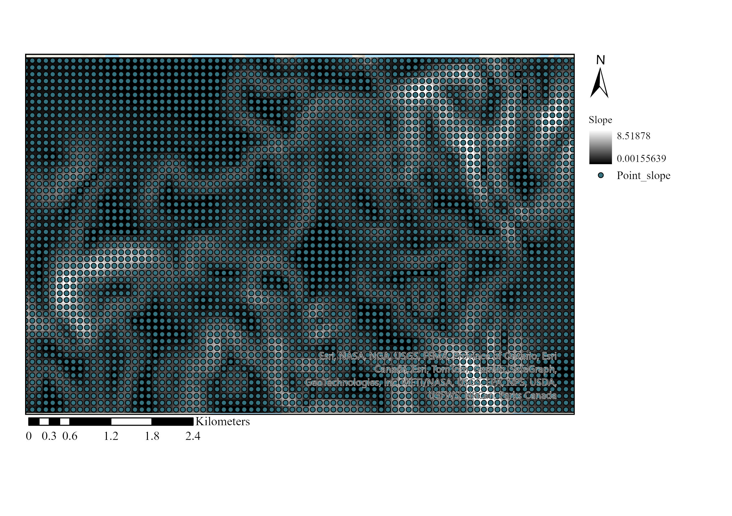
Then, I convert the slope raster to a point feature class, with each point representing the center of a cell and containing the corresponding slope value. In this image, White and black color represent slope value from the study area (raster), green dots represent slope value that has been converted to vector
1
2
3
4
5
6
7
8
9
10
11
12
#~~~~~~~~~~~~~~~~~~~~~~~~~~~~~~~STEP 4 RUN THE GENERIC FILTER and SAVE THE OUTPUT~~~~~~~~~~~~~~~~~~~~~~~~~~~~~~~~~
#generic_filter is used to run a 3x3 filter over the dem numpy array. The returned numpy array will be of the same shape as the input dem raster
slope = generic_filter(dem, calc_slope, size=3, mode='constant', # generic_filter function used to calculate the slope values for each cell in the dem array using the calc_slope function within a 3x3 window
                       cval=-9999, extra_arguments=(x_cellsize, y_cellsize)) #sets the constant value and provides additional arguments to the function while it's being applied by generic_filter function
arcpy.env.outputCoordinateSystem = input_dem.spatialReference #use the spatial reference (coordinate system) of the dem raster to set the output coordinate system

new_slope = arcpy.NumPyArrayToRaster(slope, arcpy.Point(input_dem.extent.XMin, input_dem.extent.YMin),input_dem.meanCellWidth, input_dem.meanCellHeight,-9999)
#the slope array is converted to a raster dataset by using the raster parameters (reference corner x,y coordinates, cell size, NoData value (-9999}, of the initial, dem, raster.
new_slope.save("newslope8") #the created slope raster is saved in the set workspace under the specified name

#The raster data then converted to Point
arcpy.conversion.RasterToPoint("newslope8", "slope_Point")
4. Field Management and Statistical Computation
In this setup, I first check for the existence of specific fields in the FRI feature class. If these fields exist, I delete them and create new fields for slope statistics. The script then iterates through specified PFT values, selects the relevant polygons and points, calculates statistical metrics (average, standard deviation, range) for the slope values, and updates the FRI feature class with these metrics.
1
2
3
4
5
6
7
8
9
10
11
12
13
14
15
16
17
18
19
20
21
22
23
24
25
26
27
28
29
30
31
32
33
34
35
36
37
38
39
40
41
42
43
44
45
46
47
48
49
50
51
52
53
54
55
56
57
#~~~~~~~~~~~~~~~~~~~~~~~~~~~~~~~~~~~~~STEP 5 MODIFY FIELD INSIDE FRI~~~~~~~~~~~~~~~~~~~~~~~~~~~~~~~~~~
fri = "fri" #an identifier assigns to a feature class names fri in jhf geodatabase
frifields = arcpy.ListFields (fri) #used to obtain a list of field objects associated within fri feature class
frifldsname = (f.name for f in frifields) # iterating over the field names without creating a full list of field names

fields_to_delete = ["slope_avg", "slope_std", "slope_rng"]  #create a list containing the fields that will be deleted
if fields_to_delete in frifldsname:    #checks if there is a field with the same name as the field that is getting populated
    arcpy.DeleteField_management(fri, [fields_to_delete]) #if there is such a field, it gets deleted
for field_name in fields_to_delete:
    arcpy.management.AddField(fri, field_name, "DOUBLE") #add multiple fields, loop through the fields_to_delete list and add each field individually

#~~~~~~~~~~~~~~~~~~~~~~~~~~~~~~~~~~~~STEP 6 INTERSECTING PFT AND SLOPE POINT~~~~~~~~~~~~~~~~~~~~~~~~~~~~~~
#Modify PFT Value here
pft_values = ["MCU"]


#pft_values = set(row[0] for row in arcpy.da.SearchCursor("fri", "PFT")) -----> we can also extract each unique value in PFT field to be used by using this function


for pft_value in pft_values: # initiates a loop that iterates through each unique pft_value present in the pft_values set
    query = f"PFT = '{pft_value}'" # An SQL expression used to select a subset of records, this will creates a query string that looks like PFT = 'MCU'
    selected_fri = arcpy.management.SelectLayerByAttribute(fri, "NEW SELECTION", query)  #used to select features or rows based on attribute queries in a layer

    # Iterate through selected polygons
    with arcpy.da.SearchCursor(fri, "SHAPE@") as cursor: #sets up a cursor to iterate through each row in the "fri" feature class, extracting the geometry of each feature in the form of polygons
        for row in cursor: # initiates a loop that iterates through each row in the feature class.
            polygon = row[0] # take the geometry of each feature, then store it in variable to be used in the next line

            arcpy.SelectLayerByLocation_management("slope_Point", "INTERSECT", polygon) #selects features in the "slope_Point" layer that intersect with the polygon
            point_count = int(arcpy.GetCount_management("slope_Point").getOutput(0)) #calculates the number of features present in the "slope_Point" layer and stores that count in the variable point_count

            # If more than 3 intersected points, calculate statistics
            if point_count > 3: #  If this condition is True, the next code block will be executed
                # Obtain grid_code values and populate numpy array
                grid_code_values = [] #empty list, this lit will store values from grid_code
                with arcpy.da.SearchCursor("slope_Point", "grid_code") as point_cursor: # creates a cursor (point_cursor) to iterate through the "slope_Point" to extract values from grid_code
                    for point_row in point_cursor: #loop each value in that cursor that iterates through grid_code field
                        grid_code_values.append(point_row[0]) #takes the value from the "grid_code" field and appends it to the grid_code_values list
                np_grid_code_values = np.array(grid_code_values) # converted into a NumPy array named np_grid_code_values

                # Calculate statistics
                slope_avg = np_grid_code_values.mean() #calculates the average value of the numpy array
                slope_std = np_grid_code_values.std() #calculates the standard deviation of the numpy array
                slope_rng = np_grid_code_values.ptp() #calculates the difference between max and min value (range) of the numpy array. ptp = peak-to-peak

                # Update fields in fri feature class
                with arcpy.da.UpdateCursor(fri, ["PFT", "slope_avg", "slope_std", "slope_rng"]) as update_cursor: #modified the cursor, It specifies the fields to be accessed to: "PFT", "slope_avg", "slope_std", and "slope_rng"
                    for update_row in update_cursor: #loop that iterates through each row in the fields above
                        if update_row[0] == pft_value: #checks if the value in the "PFT" field of the current row (update_row[0]) matches the pft_value.
                            update_row[1] = slope_avg  #assigns the value of slope_avg to the second field ([1]) in the list above
                            update_row[2] = slope_std  #assigns the value of slope_std to the third field ([2]) in the list above
                            update_row[3] = slope_rng  #assigns the value of slope_rng to the fourth field ([3]) in the list above
                            update_cursor.updateRow(update_row) #updates the row in the fri feature class with the modified values


                print(f"The average slope for {pft_value} is {slope_avg} degrees, the standard deviation is {slope_std}, and the range is {slope_rng}")
                break #Stop after one iteration
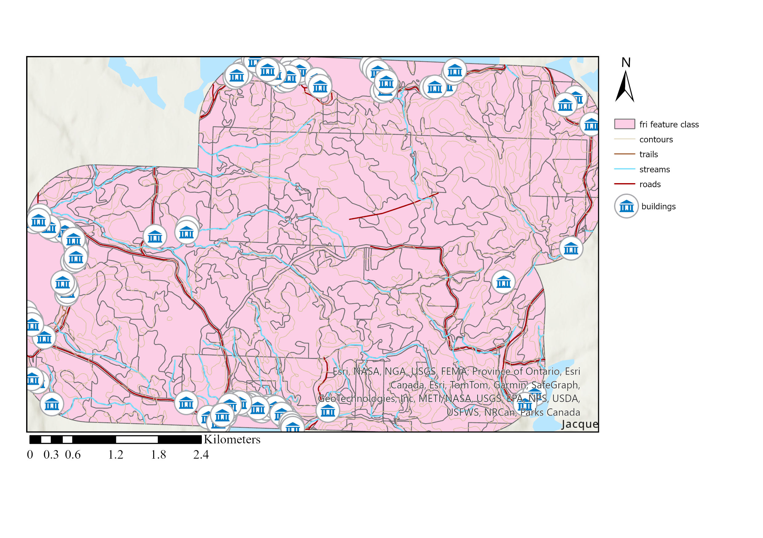 Final Map
Conclusion
The script efficiently integrates raster processing, spatial analysis, and field management within a GIS framework. It offers a flexible and user-friendly approach for analyzing slope values across different forest types. The final output includes updated fields in the FRI feature class and printed statistical metrics, providing valuable insights into the slope characteristics of various Provincial Forest Types (PFTs). Automating this process using code helps to avoid repetitive tasks, leading to increased efficiency. The potential applications of this method are vast, including environmental monitoring, land management, and urban planning.